analytical calculations
Calibration Curves: Linearity, LOD and LOQ
Building a calibration curve, judging linearity from residuals rather than r², and calculating detection and quantitation limits by the 3.3σ/S and 10σ/S conventions. A worked low-level curve and the rules for reporting results below the limit.
A limit of detection (LOD) and a limit of quantitation (LOQ) are calculated from a calibration curve as LOD = 3.3σ/S and LOQ = 10σ/S, where S is the slope of the curve and σ is the standard deviation of the response, taken from the residual standard deviation of a curve built near the limits or from the standard deviation of blank responses. ICH Q2(R2) accepts this route alongside signal-to-noise ratios of 3:1 and 10:1 and direct experimental determination 1. A calculated limit is an estimate until samples at that level have been analysed and shown to perform.
The companion reference on method validation defines linearity, range and the detection limits among the other validation parameters and says which methods need them. This page covers the arithmetic: building the curve, reading its residuals, computing the limits, and what to write when a result falls below them. The worked figures use an invented decapeptide, AGSKLEYFVR, as the analyte; they describe no real method.
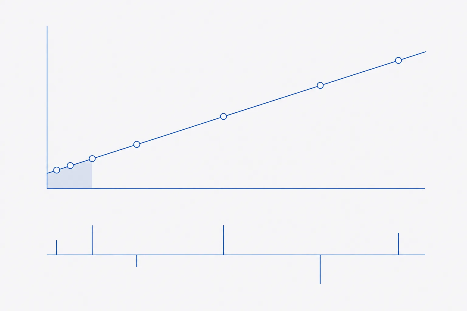
Building the curve
ICH Q2(R2) recommends a minimum of five concentrations distributed across the range for assessing linearity, a plot of the data, and the correlation coefficient or coefficient of determination, intercept and slope of the regression line, together with an analysis of the deviations of the points from the line 1. The practical requirements follow from what can go wrong.
- Define the range the curve must cover before preparing anything. For a limit test, it must reach down to the reporting level; for an assay, it must bracket the working concentration with margin on each side.
- Prepare at least five levels. Six to eight gives a more useful residual plot.
- Prepare levels as independently as practical: separate dilutions from one verified stock at minimum, and two independently weighed stocks where the budget allows. A serial chain carries one transfer bias into every level below it.
- Space levels to suit the purpose. For detection and quantitation limits, concentrate levels at the low end.
- Inject in randomised or interleaved order, not ascending, so that drift is not mistaken for curvature.
- Replicate at least the lowest and highest levels, so that the change in scatter across the range can be seen.
- Fit by ordinary least squares first, examine the residuals, and change the model only if they require it.
A worked low-level curve
Six standards of the invented peptide from 0.5 to 5 µg·mL⁻¹, detected by UV absorbance, one injection each. Illustrative figures only; peak areas are in arbitrary units.
| Concentration, µg·mL⁻¹ | Peak area | Fitted area | Residual |
|---|---|---|---|
| 0.5 | 812 | 814.3 | −2.3 |
| 1.0 | 1,570 | 1,571.4 | −1.4 |
| 2.0 | 3,105 | 3,085.5 | +19.5 |
| 3.0 | 4,555 | 4,599.5 | −44.5 |
| 4.0 | 6,160 | 6,113.6 | +46.4 |
| 5.0 | 7,610 | 7,627.7 | −17.7 |
The residual standard deviation is the square root of the sum of squared residuals divided by n − 2, here with four degrees of freedom: 34.78 area units. It is the σ used below. The residuals change sign without a run of same-signed values and show no systematic trend with concentration, so a straight line is an adequate model over this range.
Why r² is not a test of linearity
The coefficient of determination measures how much of the variation in response is explained by the line. Across a wide range, almost any monotonic relationship explains most of it. A detector response that flattens by a few per cent at the top of the range can still return r² above 0.999, while the top standard reads several per cent low and every sample near it is biased. ICH Q2(R2) asks explicitly that any non-random pattern in the residuals be assessed, and that linearity assessment include how the error changes across the range 1.
| Pattern in the residual plot | Indicates | Response |
|---|---|---|
| Random scatter of constant width about zero | Straight line adequate, variance constant | Accept ordinary least squares |
| Arc: negative at both ends, positive in the middle, or the reverse | Curvature | Narrow the range, or justify a quadratic model |
| Funnel: scatter widening with concentration | Variance increases with level | Weighted regression, typically 1/x or 1/x² |
| One point far from the rest | Preparation or injection error at that level | Investigate and re-prepare; do not simply delete |
| Steady drift with injection order | Instrument drift, not a property of the curve | Randomise order; check system suitability |
The funnel pattern matters most for low-level work. With unweighted regression, the large absolute scatter at high concentrations dominates the fit, and the line can pass wide of the low standards in proportional terms. Where the curve must serve near the LOQ and far above it, either weight the regression or build a separate low-level curve, which is the approach taken here.
The intercept
A non-zero intercept is normal and is not by itself a defect. It is compared with its own standard error; if the confidence interval includes zero, the intercept is not significantly different from zero. Forcing the line through the origin when the data do not support it biases the slope and moves every low result. Here the intercept of 57.29 is small beside the response at the lowest standard, and is retained in the model.
Reading a sample from the curve inverts the fitted line: concentration = (response − intercept) ÷ slope. A sample peak area of 2,850 gives (2,850 − 57.29) ÷ 1,514.08 = 1.84 µg·mL⁻¹. The uncertainty of a value read this way is smallest near the centre of the calibrated range and grows towards both ends, because the confidence band around a regression line widens away from the mean of the standards. Samples are therefore best diluted to fall near the middle of the curve, and results from the extreme standards deserve the least confidence.
Detection and quantitation limits
The IUPAC definition of the limit of detection starts from the blank: the smallest measure detectable with reasonable certainty is the mean of the blank measures plus k times their standard deviation, with k chosen for the confidence required, and the limit in concentration follows through the calibration function 3. Currie's framework, adopted by IUPAC in 1995, separates the decision level at which a signal is judged present from the detection limit at which it will reliably be found, and defines a quantification limit by a target relative standard deviation 2.
The ICH convention condenses this. The factor 3.3 is approximately twice 1.645, the one-sided 95% point of the normal distribution, and so allows for false positives and false negatives at about 5% each. The factor 10 corresponds to a relative standard deviation of about 10% at the quantitation limit. For σ, ICH accepts the residual standard deviation of a regression line or the standard deviation of y-intercepts of regression lines, from a curve evaluated with samples in the range of the limits 1. A σ taken from a curve spanning the whole working range is inflated by high-level scatter and overstates both limits.
| Limit | Formula | Calculation | Result |
|---|---|---|---|
| Detection limit | 3.3σ/S | 3.3 × 34.78 ÷ 1,514.08 | 0.076 µg·mL⁻¹ |
| Quantitation limit | 10σ/S | 10 × 34.78 ÷ 1,514.08 | 0.23 µg·mL⁻¹ |
| Quantitation limit, molar | QL ÷ M | 0.2297 µg·mL⁻¹ ÷ 1,169.35 g·mol⁻¹ | 0.20 µmol·L⁻¹ |
Both calculated limits lie below the lowest standard of 0.5 µg·mL⁻¹, so they are extrapolations. ICH Q2(R2) expects a limit obtained by calculation or extrapolation to be supported by analysis of samples near or at that level 1. In practice, prepare six or more samples at the calculated LOQ and confirm that accuracy and precision meet the stated criteria there. If they do not, the LOQ is the lowest level at which they do, not the calculated figure.
Signal-to-noise alternative
For methods with a visible baseline, such as chromatography with UV detection, the limits can instead be set from signal-to-noise. Signals from samples of known low concentration are compared with blank signals or with a baseline region near where the peak elutes; a ratio of 3:1 is generally acceptable for the detection limit and at least 10:1 for the quantitation limit 1. The noise measurement must be defined in the procedure — the window width and whether noise is measured peak to peak — since different conventions give results differing by about a factor of two 4.
Reporting results near and below the limits
A response between the LOD and the LOQ shows that the analyte is present but does not support a reliable figure. A response below the LOD does not show absence; it shows that the method could not tell. Both must be reported with the limit that applies.
| Measured result | Region | Report as |
|---|---|---|
| 1.84 µg·mL⁻¹ | At or above LOQ | The value, rounded to the reporting place |
| 0.15 µg·mL⁻¹ | Between LOD and LOQ | Detected, below LOQ (0.23 µg·mL⁻¹); the value may be given for information, flagged as estimated |
| 0.04 µg·mL⁻¹ | Below LOD | Not detected (below 0.076 µg·mL⁻¹) |
| Any result | Outside the validated range at the top | Dilute into range and reanalyse; do not extrapolate |
Zero is never a correct report for a result below the limits, and neither is a blank field. Both are later read as measured absence, and both are summed as zero into totals where they may not belong. For impurity methods, the QL must be at or below the reporting threshold, or the method cannot report what it is required to report 1.
Procedure
- Write the purpose and required range, including the lowest level that must be reported.
- Prepare at least five independently derived levels; weight the low end where limits are needed.
- Inject in randomised order, with replicates at the extremes.
- Fit by least squares and plot residuals against concentration. Act on structure, not on r².
- Choose the model and weighting the residuals support, and record why.
- Compute σ from a low-level curve or blank replicates, then LOD = 3.3σ/S and LOQ = 10σ/S; or determine signal-to-noise under a defined noise convention.
- Confirm the LOQ with six or more samples at that level against predefined accuracy and precision criteria.
- State the limits and the convention used in the procedure and on every report that relies on them.
Limits are properties of a method on an instrument at a time. A new column, a new detector lamp or a new analyst can move them, and a limit stated without its date and conditions carries less information than it appears to 4.
References
- ICH Q2(R2) Validation of analytical procedures — Scientific guideline
- Nomenclature in evaluation of analytical methods including detection and quantification capabilities (IUPAC Recommendations 1995)
- limit of detection (L03540)
- The Fitness for Purpose of Analytical Methods: A Laboratory Guide to Method Validation and Related Topics, second edition