stability study design
Accelerated Stability and Arrhenius Extrapolation: What a Hot Study Can and Cannot Predict
The Arrhenius equation, what the activation energy silently assumes, a worked extrapolation from three temperatures, why lyophilised and solution peptides break the model in different ways, and what ICH allows an accelerated result to support.
Only within limits the study has to establish for itself. An accelerated study measures degradation rates at elevated temperature; the Arrhenius equation converts them into a rate at the storage temperature, on the assumption that the same reaction, with the same activation energy, governs loss across the whole range. Where that holds, the prediction can be good, and for many solid small-molecule products it has been shown to be 12. Peptides break the assumption in characteristic ways — through changes of route, of physical state and of pH with temperature — and the breaks are larger in solution than in a dried solid 5.
This entry is the chemistry of extrapolation. Where the accelerated arm sits inside a full study is covered in the stability study design entry; which degradation routes are operating is covered in the degradation entries of this handbook.
The equation
The Arrhenius equation states that a rate constant k depends on absolute temperature T as k = A·exp(−Ea/RT), where Ea is the activation energy, R the gas constant, 8.314 J/(mol·K), and A the pre-exponential factor. Taking logarithms gives a straight line: ln k = ln A − (Ea/R)(1/T). Plot ln k against 1/T and the slope is −Ea/R. Temperatures must be in kelvin; a plot in degrees Celsius is not a straight line 1.
For extrapolation the ratio form is the useful one. The rate at a hot temperature T1 divided by the rate at a cold temperature T2 is exp[(Ea/R)(1/T2 − 1/T1)]. The ratio depends on nothing but the activation energy and the two temperatures, so the choice of Ea decides the answer.
| Activation energy | 40 °C over 25 °C | 25 °C over 5 °C | 40 °C over 5 °C |
|---|---|---|---|
| 50 kJ/mol | 2.6 | 4.3 | 11 |
| 80 kJ/mol | 4.7 | 10 | 48 |
| 110 kJ/mol | 8.4 | 24 | 204 |
Read the last column. Across a plausible range of activation energies, one month at 40 °C stands for anything from about eleven months to about seventeen years at 5 °C. The familiar rule that a reaction doubles or triples in rate for every 10 °C rise is the same equation with Ea fixed at a middling value; it gives a factor of roughly eleven to forty-seven over the same interval and conceals exactly the uncertainty that matters 1.
What the activation energy assumes
A single straight line through ln k against 1/T carries four assumptions. The loss is governed by one rate-limiting reaction, or by several with similar activation energies. That reaction does not change mechanism over the range. The system does not change physical state over the range. And the rate being fitted is the rate of the attribute that actually limits the period 16.
The first assumption fails most quietly. When two routes run in parallel with different activation energies, the route with the higher activation energy speeds up more on heating and slows down more on cooling. A hot study is therefore dominated by high-activation-energy routes, and a low-activation-energy route that is minor at 40 °C can be the main route at 5 °C. The fitted line then describes a reaction that is not the one limiting storage, and the extrapolation is optimistic.
| Assumption | How it fails for peptides | Effect on the prediction |
|---|---|---|
| One dominant route | Hydrolysis, deamidation, oxidation and aggregation run together with different activation energies | Usually optimistic: the route that matters cold is underweighted hot |
| Constant mechanism | Conformational change or loss of structure above a threshold opens new routes, aggregation in particular | Pessimistic if the hot route never operates cold; misleading either way |
| Constant physical state | A dried cake passes its glass transition; a solution freezes; an excipient melts or crystallises | Invalid across the transition in either direction |
| Constant solution conditions | Buffer pH shifts with temperature, by roughly 0.03 pH units per degree for amine buffers such as Tris | The hot arm is at a different pH from the cold one |
| Constant water content | A solid gains or loses moisture differently at each condition | Rate tracks humidity as well as temperature |
Lyophilised and solution: two different failures
In a dried solid the governing variables are temperature, residual moisture and molecular mobility. Water is a plasticiser, so the glass transition temperature of an amorphous cake falls as it takes up moisture; a humid accelerated condition can push the cake above its glass transition, where mobility and rate rise far faster than the equation predicts 5. Waterman and colleagues addressed the moisture term directly with a humidity-corrected form, ln k = ln A − Ea/RT + B·RH, where B measures sensitivity to relative humidity, fitted from short studies across several temperature and humidity combinations 2. Their accelerated stability assessment programme also replaced the rate with isoconversion: the time taken to reach the specification limit at each condition, which avoids assuming a reaction order.
In solution the failures are about structure and chemistry. Peptides that hold secondary structure can lose it on heating, exposing new sites to attack and promoting association, so a route that barely exists at 5 °C can dominate at 40 °C 5. pH drifts with temperature in most buffers. Dissolved oxygen falls as temperature rises, which slows oxidation in the hot arm relative to the cold one. And no extrapolation from above 0 °C describes frozen storage: freezing concentrates solutes in the unfrozen fraction and introduces ice interfaces, so the chemistry below the freezing point is not the chemistry above it.
The consolidated ICH Q1 draft states the same distinction in regulatory terms. It notes that a solid synthetic product may follow the humidity-modified Arrhenius equation for its limiting attributes, while biological products may be less amenable to that kind of modelling, and it treats physical attributes as case by case. The draft groups chemically synthesised polypeptides with the synthetic entities for its purposes, which places many research peptides on the modelling-friendly side of that line on paper; their physical behaviour in solution still has to be checked rather than assumed 4.
A worked extrapolation
The figures below are invented to show the arithmetic. They describe no real material. Assay loss is small enough over the study to be treated as linear in time, so each rate is a loss in percentage points of assay per month.
- Measure the rate at three temperatures: 0.50 per month at 40 °C, 1.29 at 50 °C and 3.16 at 60 °C.
- Convert to kelvin and take reciprocals: 0.003193, 0.003095 and 0.003002 per kelvin.
- Take natural logarithms of the rates: −0.693, 0.258 and 1.152.
- Fit ln k against 1/T. The slope is about −9,620 K, so Ea is 9,620 × 8.314, or about 80 kJ/mol.
- Predict the rate at 25 °C from the fitted line: about 0.107 per month. A 5-point loss takes about 47 months.
- Predict the rate at 5 °C: about 0.0105 per month. A 5-point loss takes about 478 months, roughly 40 years.
- Repeat the 5 °C prediction at the edges of a plausible activation-energy range. At 50 kJ/mol the 5-point loss takes about 112 months; at 110 kJ/mol, about 2,040.
- Check the degradant profile at each temperature. If the 60 °C samples show a peak absent at 40 °C, drop the 60 °C point and report that the fit rests on two temperatures.
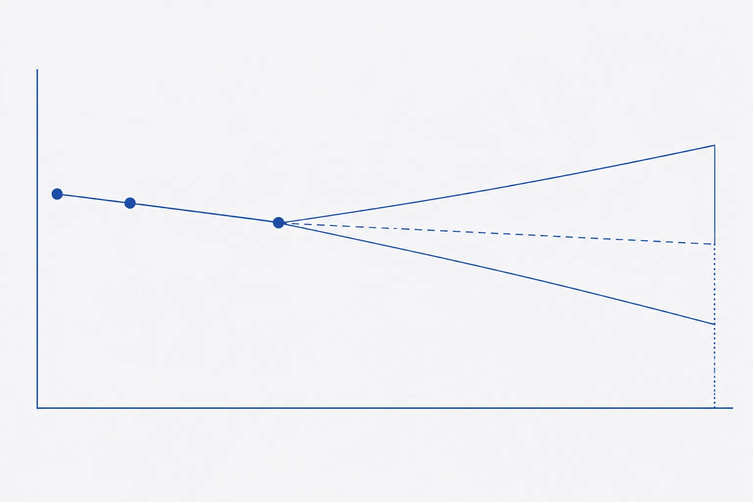
Three observations follow. Three points with modest scatter fix the slope loosely, and the error in the slope is multiplied by the length of the extrapolation; the uncertainty on a 5 °C prediction from 40 to 60 °C data is wide even when the fit looks clean, which is why the fitting method itself has been examined as a source of error 6. A prediction of forty years from six months of data is a statement about the model, not the material. And the result at 25 °C is far better supported than the result at 5 °C, because it sits much nearer the measured range.
What ICH allows an accelerated result to support
Under Q1A(R2) the accelerated condition supports the long-term data and reveals sensitivity to excursions; it does not set the period. For refrigerated material, significant change between three and six months at 25 °C means the period rests on real-time data at the long-term condition, and significant change within the first three months calls for a discussion of what short excursions do 3. Q1A(R2) permits only limited extrapolation of real-time data beyond the observed range, justified by the degradation mechanism, the accelerated results and the goodness of fit, and states plainly that it assumes the same degradation relationship continues 3.
Q1E sets how far that extrapolation may go. Where there is no significant change at the accelerated condition, a proposed period can at most be twice the period covered by long-term data and no more than 12 months beyond it; for material stored in a refrigerator, at most one and a half times and no more than 6 months beyond. Where the accelerated condition does show significant change, the period depends on the results at the intermediate and long-term conditions, not on the accelerated data 7. The consolidated draft adds an annex on enhanced stability modelling, under which a qualified model built on prior knowledge and accelerated data may support a period beyond the real-time data, with the model's scope, verification and maintenance documented 4. Neither text treats a single Arrhenius fit as enough by itself.
Using a hot study honestly
- Use at least three elevated temperatures, spaced widely enough to define a slope.
- Keep every temperature below known transitions: the glass transition of the cake at the study humidity, any structural transition in solution, and any excipient melting point.
- Control or record humidity for solids, and fit a humidity term if more than one humidity is used.
- Fit the attribute that limits the period: a named degradant or the assay, not total purity by default.
- Compare the degradant profile at each temperature. A different profile is a different reaction and cannot share the line.
- Report the activation energy with its confidence interval and carry that interval through to the prediction.
- Never extrapolate across freezing. Frozen storage is established by real-time data at the frozen condition.
- Label the result provisional, run real-time pulls alongside, and replace the prediction with data as they arrive.
An accelerated study is at its best as an early warning and a ranking tool. It shows quickly which formulation, container or lot is least stable, and whether a material is sensitive enough to temperature for an excursion to matter. It is at its weakest as a substitute for time. The period a material can be held for is established at the condition it is held at 35.
References
- Accelerated aging: prediction of chemical stability of pharmaceuticals
- Improved protocol and data analysis for accelerated shelf-life estimation of solid dosage forms
- ICH Q1A(R2) Stability Testing of New Drug Substances and Products
- ICH Q1 Stability Testing of Drug Substances and Drug Products — Step 2 draft guideline
- Stability of protein pharmaceuticals: an update
- A scientific and statistical analysis of accelerated aging for pharmaceuticals. Part 1: accuracy of fitting methods
- ICH Q1E Evaluation for Stability Data