Mass Balance in Forced Degradation: Calculation and Shortfalls
The reconciliation a stability-indicating method depends on: the ICH Q1A(R2) definition, the (assay + degradants) ÷ initial formula normalised to the unstressed sample, response-factor and molecular-weight corrections worked for a generic stressed peptide, how the acceptance window follows from precision, and the numbered investigation when degradants are missing.
Mass balance in a forced-degradation or stability study is the process of adding together the assay value and the levels of degradation products to see how closely they add up to 100 % of the initial value, with due consideration of the margin of analytical error; that is the glossary definition in ICH Q1A(R2) 1. As a calculation: mass balance (%) = (assay of the stressed sample + corrected total degradants) ÷ (assay of the unstressed sample + its related substances) × 100, with every term expressed as per cent by weight of the initial material. ICH gives no acceptance figure. Laboratories derive a window from the method's precision, and fixed windows of about 97 to 103 % or 95 to 105 % are in common use. A result below the window means material has left the measurement: a degradant that does not elute, does not absorb at the detection wavelength, has precipitated or adsorbed, or is volatile.
Companion references cover the design of a forced-degradation study and what makes a method stability-indicating. This page covers the reconciliation both rely on. The worked example is an invented 13-residue peptide of molar mass 1,420.6 g·mol⁻¹, subjected to oxidative stress; all figures are illustrative and describe no real material.
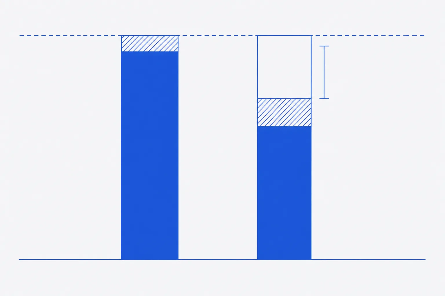
The ICH Q1A(R2) definition of mass balance
Q1A(R2) places stress testing at the start of stability work: it identifies the likely degradation products, establishes the degradation pathways and validates the stability-indicating power of the analytical procedures 1. Mass balance is the quantitative half of that validation. If the purity method sees every product the assay loss implies, the two methods agree and the method is shown to be stability-indicating for that route of degradation. If they do not agree, the method is missing something, and the guideline's instruction to review the adequacy of the mass balance when evaluating stability data is the point at which the gap must be explained 1.
The phrase due consideration of the margin of analytical error is the whole of the guideline's acceptance criterion. It means the window is a property of the method's precision, not a fixed number, and that a shortfall is judged against the uncertainty of the difference between two measured sums. The section on acceptable range below works that out.
The basic formula and its normalisation to the unstressed sample
Normalise to the unstressed sample rather than to a nominal 100 %. The starting material already contains related substances and may assay below 100 % against the reference standard on an as-is basis; dividing by its own assay plus related substances removes both the standard's assigned value and the moisture and counterion content from the comparison. Prepare and analyse the stressed and unstressed samples together, on the same day against the same standard, so that systematic errors in the standard, the dilution and the detector cancel.
The terms must share a basis. The assay is per cent by weight of initial content, from an external standard. Degradants are quantified against the parent reference standard, which puts them on the same basis only if each is corrected for its response factor and all of them elute. A total degradant figure read as area per cent is not on that basis and cannot be added to an assay value; the companion reference on stability-indicating methods explains why area normalisation can read 100 % while material is being lost.
Correcting for response factors and molecular weight
Two corrections convert a degradant's measured response into parent lost. The first divides by its relative response factor, so that a species absorbing less than the parent is not under-counted; RRFs come from impurity standards or, where none exists, from a formula-based detector such as the chemiluminescent nitrogen detector paired with UV, which Nussbaum and colleagues showed yields relative UV response factors without isolating the impurity 3. The second multiplies by the ratio of molar masses, M(parent) ÷ M(degradant), because one mole of parent lost produces one mole of degradant, and a heavier degradant therefore weighs more than the parent it came from. Lukulay and Hokanson showed that the error from ignoring the mass ratio grows with the mass difference and is nearly independent of the degradant level, so it is worth applying even at low levels 2.
| Correction | Formula | Matters most when |
|---|---|---|
| Response factor | Mass % = measured % against parent ÷ RRF | The degradant has lost or gained a chromophore: fragments without aromatic residues, tryptophan oxidation products, adducts |
| Molecular weight | Parent-equivalent % = mass % × M(parent) ÷ M(degradant) | The degradant mass differs from the parent by more than a few per cent: adducts, dimers, large excipient conjugates |
| Cleavage pair | Parent-equivalent % = (mass % of both fragments) × M(parent) ÷ (M(parent) + 18.0) | Hydrolysis gives two fragments whose masses sum to the parent plus water; correct the pair once, not each fragment |
Worked example for a generic peptide stress sample
Invented 13-residue peptide, M = 1,420.6 g·mol⁻¹, containing one methionine and the aromatic residues clustered in the C-terminal half. Oxidative stress produced a sulfoxide, a sulfone and a hydrolytic cleavage pair. Assay by external standard at 214 nm; degradants quantified against the parent standard at the same wavelength, initially with every RRF taken as 1.
| Degradant | Measured % (RRF = 1) | RRF | ÷ RRF | M (g·mol⁻¹) | Parent-equivalent % |
|---|---|---|---|---|---|
| D1: methionine sulfoxide (+16) | 5.60 | 1.02 | 5.490 | 1,436.6 | 5.429 |
| D2: methionine sulfone (+32) | 0.90 | 1.02 | 0.882 | 1,452.6 | 0.863 |
| D3: fragment, residues 1 to 6 (no aromatic residues) | 1.00 | 0.62 | 1.613 | 702.8 | 2.182 (pair) |
| D4: fragment, residues 7 to 13 (both aromatic residues) | 0.80 | 1.34 | 0.597 | 735.8 | included in pair |
| Related substances unchanged from the unstressed sample | 0.70 | 1.00 | 0.700 | 0.700 | |
| Total degradants | 9.00 | 9.282 | 9.174 |
| Stage | Total degradants (%) | Assay + degradants (%) | Mass balance (%) |
|---|---|---|---|
| Uncorrected | 9.00 | 96.30 | 96.30 ÷ 99.8 = 96.5 |
| RRF-corrected | 9.28 | 96.58 | 96.58 ÷ 99.8 = 96.8 |
| RRF and molecular-weight corrected | 9.17 | 96.47 | 96.47 ÷ 99.8 = 96.7 |
The corrections move the figure by 0.2 of a point and then back by 0.1. That is the normal size for a peptide at 214 nm: response per unit mass is dominated by the backbone and so stays near 1 except where the aromatic residues are partitioned, and the mass changes from oxidation are small against a molar mass of 1,400. The two fragments illustrate the one place the RRF correction is large and why it must be applied to the pair as a whole: D3 reads low and D4 reads high, and only their corrected sum, 2.21 %, is the mass of parent that was cleaved.
What remains after correction is a shortfall of 99.8 − 96.47 = 3.3 points of the initial material. Correction has not explained it. The next section decides whether it is large enough to investigate.
What range is acceptable and why it depends on precision
Mass balance is a difference between two sums, each of an assay and a total degradant figure. Its standard uncertainty is the root of the sum of squares of the four contributions. With a standard uncertainty of 0.6 % on each assay, 0.4 % on the stressed total degradants and 0.1 % on the unstressed related substances, u = √(0.6² + 0.4² + 0.6² + 0.1²) = 0.94 %, and the expanded uncertainty at k = 2 is 1.9 %. For this method, a mass balance between 98.1 and 101.9 % is indistinguishable from 100 %; the worked figure of 96.7 % lies 1.4 points outside that window and cannot be attributed to analytical error.
A fixed window, used without this calculation, is a compromise. Set wider than the method's expanded uncertainty it lets real losses through; set narrower it generates investigations of noise. Reviews of forced-degradation practice treat mass balance as one of the criteria by which a method is accepted as stability-indicating, alongside specificity and peak purity, and note that it is routinely assessed in the range of a few per cent around 100 5. Alsante and colleagues place the same check inside degradant profiling: the products identified and quantified must account for the parent lost before the profile is considered complete 4. The following table turns the uncertainty into actions.
| Shortfall from 100 % | Reading | Action |
|---|---|---|
| Within U | Consistent with analytical error | Record; no further action |
| Between U and 2U | Marginal | Re-prepare and re-analyse both samples; check sample history and dilution records |
| Beyond 2U | Material unaccounted for | Open the shortfall investigation below |
| More than about 5 points | A major product is not being measured, or material has left solution | Orthogonal detection and a recovery check before any further stress work |
Causes of shortfall: elution, absorptivity, solubility, volatility
| Cause | Mechanism | Sign on the data | First check |
|---|---|---|---|
| Does not elute | Covalent aggregate or adsorbed species retained on the column, or eluting after the gradient ends | Rising back-pressure; ghost peaks in the next blank; late broad hump | Extend the gradient, run a strong-solvent wash and integrate it; size-exclusion chromatography |
| Does not absorb | Small fragments with few peptide bonds elute in the solvent front; at 280 nm anything without tryptophan or tyrosine is invisible | Assay loss with no new peaks; shortfall grows with stress time | Mass spectrometry, charged aerosol or nitrogen-specific detection |
| Not in solution | Precipitate, insoluble aggregate or adsorption to the vial, filter or needle | Haze; shortfall that varies between replicate preparations; loss of both assay and degradants | Inspect the vial; analyse the filter and the vial residue; recovery check |
| Volatile or lost to headspace | Small polar fragments or ammonia from deamidation in open containers | Shortfall that grows with handling time, not stress time | Closed containers; headspace analysis |
| Mis-quantified | Co-elution with the parent, isomers of identical mass, wrong RRF, wrong wavelength | Assay too high; degradants that appear and vanish; corrected total moving in the wrong direction | Peak purity by mass spectrometry; re-determine RRFs; second wavelength |
Investigating a shortfall: orthogonal detection and recovery checks
- Confirm the arithmetic and the basis: same reference standard, same day, assay and degradants both as per cent by weight of initial, every RRF and molar mass entered as recorded.
- Check the sample history: container, dilution, filter, hold time and temperature between stress and injection. Prepare fresh stressed and unstressed samples and repeat.
- Extend the gradient to full organic and hold; run a strong-solvent column wash into the detector and integrate everything that elutes. Compare the total area with the unstressed sample.
- Re-run with a detector that does not depend on the chromophore: mass spectrometry for identity, charged aerosol or nitrogen-specific detection for amount. Look in the solvent front for small fragments.
- Recovery check: analyse the stressed solution by size-exclusion chromatography for soluble aggregate; dissolve any residue from the vial and filter in strong solvent and analyse it; compare recovered mass with the expected total.
- Re-examine each degradant's RRF and molar mass, and confirm that cleavage pairs have been corrected once.
- If a product is found, extend the method to measure it, recompute the mass balance and record the revised figure. If none is found, record the limit of the method as a documented gap rather than adjusting any number.
For the worked example, the pattern of a 3.3-point shortfall that survives correction, with no new peaks and an unchanged chromatogram, points first to non-eluting or insoluble material: the size-exclusion run and the vial-residue analysis are the decisive steps. In a peptide study that is the common finding, because oxidative and interfacial stress both promote aggregation, which the companion reference on aggregation treats in full.
Documenting mass balance in the study report
- The definition and formula applied, with the normalisation basis stated.
- Assay and total degradants for the unstressed and each stressed sample, as per cent by weight of initial, with the reference standard and date.
- Each degradant's RRF, its source and date, and its molar mass or the pair it belongs to.
- The uncorrected, RRF-corrected and fully corrected mass balance for each stress condition.
- The method's expanded uncertainty for the mass-balance difference and the window derived from it.
- Every shortfall beyond the window, the investigation steps taken, what was found and the revised figure, or the documented gap.
A mass balance of 99.6 % recorded without its uncertainty or its corrections is a number. A mass balance of 96.7 % recorded with both, and with the investigation that followed, is evidence about what the method can and cannot see. The second is the one a stability study needs.
References
- ICH Harmonised Tripartite Guideline Q1A(R2): Stability Testing of New Drug Substances and Products
- Reconciling Mass Balance in Forced Degradation Studies
- Determination of relative UV response factors for HPLC by use of a chemiluminescent nitrogen-specific detector
- The role of degradant profiling in active pharmaceutical ingredients and drug products
- Development of forced degradation and stability indicating studies of drugs — A review